
How to create a Pivot Table in Excel
A pivot table is a tool in Excel that allows you to quickly summarize data in your spreadsheet.
A pivot table is a tool in Excel that allows you to quickly summarize data in your spreadsheet.
1
Step 1 of 16Here we have a table of data containing order information.
Let's use a pivot table to summarize this information and display the total quantity for each order.
test
2
Step 2 of 16To get started, highlight the cell where you'd like to create the pivot table.
In this example we've selected cell A1 on sheet 2.
3
Step 3 of 16Next, select the Insert tab from the toolbar at the top of the screen.
4
Step 4 of 16In the Tables group, click on the Pivot Table button.
5
Step 5 of 16A window called Create Pivot Table should appear. Select the range of data for the pivot table.
6
Step 6 of 16In this example we'll select cells A1 to F16 in sheet 1.
7
Step 7 of 16This will be the source of data for the pivot table. Now click on the OK button.
8
Step 8 of 16A blank pivot table should now appear on sheet 2 of your spreadsheet.
9
Step 9 of 16Next we will choose the fields to add to the pivot table.
10
Step 10 of 16To add order ID and quantity, select the checkboxes next to these fields.
11
Step 11 of 16By default these fields are added to the pivot table as summed values.
12
Step 12 of 16Since we would rather see each order ID individually as a row in our pivot table, we will drag Sum of Order ID from the Values section to the Rows section.
13
Step 13 of 16Now each order ID is displayed as a row in the pivot table.
14
Step 14 of 16However, Excel has defaulted the title in cell A1 to say Row Labels.
15
Step 15 of 16Let's change the title to something more meaningful, such as Order ID.
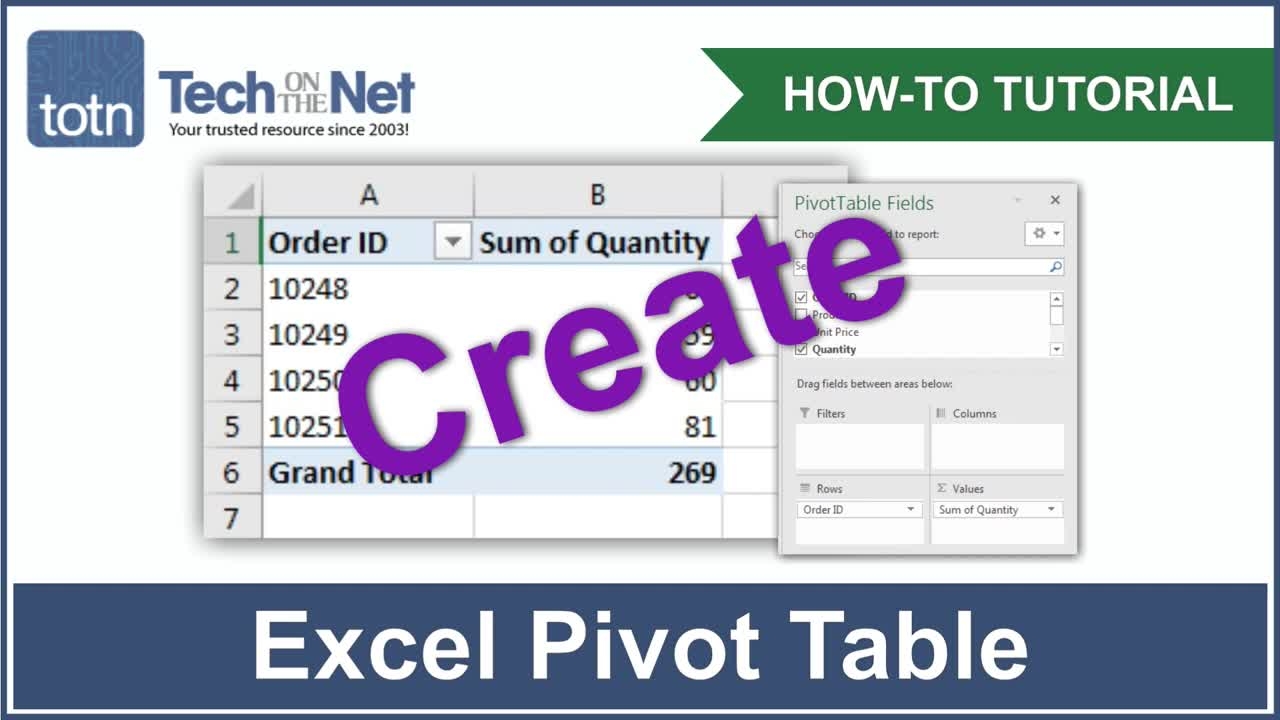
Our pivot table now shows all of the order information summarized.
16
Step 16 of 16We can see the order ID values displayed in rows with the total quantity for each order.